Lab Notes: TensorFlow for Time Series Prediction, Part 3 – LSTMs & Multi-Step Forecasts

In the previous article in this series, we built a simple single-layer neural network in TensorFlow for time series prediction, forecasting values based on a time series dataset. . We saw that by taking in a window of prior data, we could train our single hidden neuron to take in 30 values, apply weights to them, and add a bias to produce predictions for the next value in the series. We also broke time series data down into the characteristics of trend (continuous movement in one direction), seasonality, (repeated patterns with consistent time windows), and noise (unpredictable variations). In this article, we’ll try using Recurrent Neural Networks (RNNs), which are specialized for predicting sequences. Specifically, we’ll look at Long Short-Term Memory Networks (LSTMs), which are more specialized in learning and predicting events in a time series. If you’d like to follow along with the code, this article is also available via Google Colab.

← View previous articles in this series:
• TensorFlow for Time Series Prediction, Part 1 – Hello World
• TensorFlow for Time Series Prediction, Part 2 – Working with Time Series

Feed-Forward Networks

Previously, our simple neural network took in a window of 30 data points, and made a prediction for the next point in the series. We can define this as a single-step model, as it’s only outputting a single point of the time series, despite taking in a series of inputs. While this type of prediction is useful in some cases, there are many times where we’d prefer to predict an entire sequence of data as our output. For instance, weather prediction systems will often give predictions for an entire week into the future, using a combination of current and historical data to produce the time series. We can define models that produce sequences of output as multi-step models.

To refresh, let’s look back at the networks we’ve trained so far. Training a standard, feed-forward network involves the following steps:

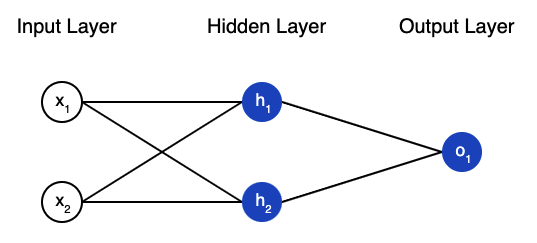
1. We input an example of labeled data from the dataset.
2. This input is fed into the network through an input layer made up of neurons, where the number of neurons is equal to the dimensionality of the input data.
3. The input layer connects to a hidden layer of neurons via edges, each with its own weight. The summation of these weighted input values, plus a bias, sets the value of the hidden neuron.
4. These neurons feed into one another across hidden layers until reaching the output layer, where a value or prediction is produced.
5. Comparing the prediction against the true value produces an error. This is then propagated back through the network to adjust the weights and biases.
6. We iterate this process for a set number of epochs, and then test the trained network against new data.

We implemented a single hidden layer with one neuron for training. Expanding this to a Deep Neural Network (DNN) simply involves adding additional hidden layers, each with a specified number of neurons. While there’s tons of intuition and trial and error in determining the best architecture for a deep neural network, we’ll leave that to the textbooks.

Recurrent and LSTM Networks

When it comes to predicting sequences, feed-forward neural networks have a number of pitfalls:

1. They cannot handle sequential data. If you remember, we trained our time series prediction model on shuffled-up data. The actual order of the sequence wasn’t even taken into account when training!
2. They consider only the current input.
3. They cannot memorize previous input.

A Recurrent Neural Network (RNN) addresses these issues by having its hidden layers take in both the current input, which we’ll call x1, in addition to the output of the hidden layer from the last input, which we’ll call h0.

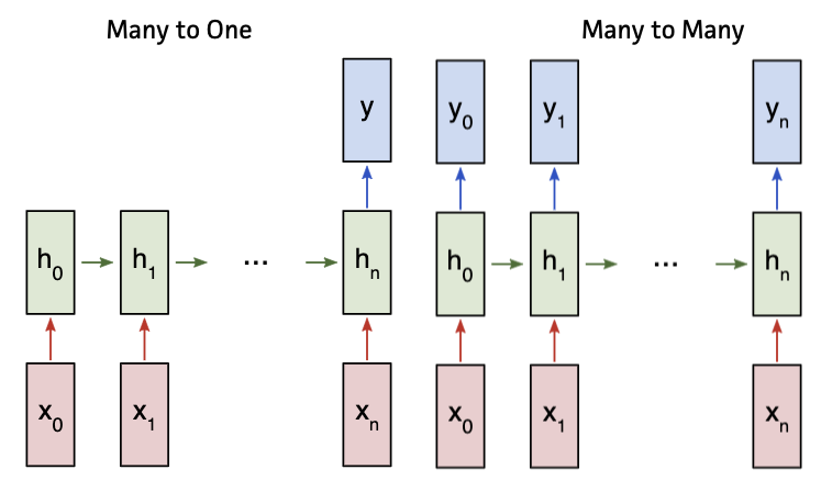
By feeding the output of one layer into the input of the next, RNNs factor in previous inputs, and become better at recognizing sequences of multiple inputs across time. They’re also capable of producing a full output sequence (many-to-many), or a single output (many-to-one), from the input sequence. While this can lead to better time series prediction, simple RNNs have a common pitfall known as the vanishing gradient problem. When propagating across the timestamps in the RNN to train the network, the impact of previously hidden layer values decreases as the layers get further apart. With some tasks, we need to consider the context from many time-stamps ago, and any crucial context can get lost due to being too distant in the past. With time series, this can really hurt the accuracy when learning seasonal patterns with large gaps of time in-between.

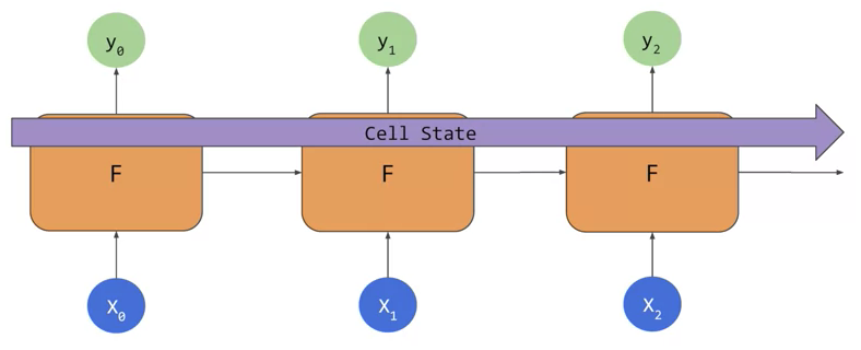
Thankfully, there’s a special kind of RNN uniquely suited to learning long-term dependencies. Long Short-Term Memory (LSTM) networks were designed specifically to address the vanishing gradient problem. LSTMs store a cell state that propagates across the sequence of inputs, in addition to the context being passed forward by traditional RNNs. This helps keep context from earlier inputs relevant across the entire series.

Building our Time Series Prediction

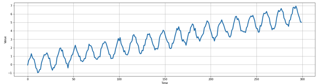
Let’s explore how both a DNN and LSTM network can forecast a time series. To begin, we’ll construct a time series similar to before, with a clear trend and seasonality, as well as some random noise. To keep it simple, our time series will be a rising sine wave with some random noise applied.

for time in range(0, total_steps, 1):
   val = trend(time, slope)
   val += sine_wave(time)
   val += white_noise(0.3)
   series.append(val)
. . .
df = pd.DataFrame({"series": series[0:steps]}, columns=["series"])
df_test = pd.DataFrame({"series": series[steps:]}, columns=["series"])
 
# Visualizing the data
plot_series(df[["series"]])

Next, we’ll preprocess our data to values in the range between 0 and 1. This is a common practice in machine learning problems for improving model accuracy. Given that the relative values of each data point will remain the same, we can train our model on this processed dataset, and then convert back to true values for our predictions. We’ll do this using the RobustScaler class from Scikit Learn.

from sklearn.preprocessing import RobustScaler
. . .
# Transform the data by scaling each feature to a range between 0 and 1
scaler = RobustScaler()
np_data_scaled = scaler.fit_transform(np_data_unscaled)

In the previous article, we divided our data between a training set, which was fed into our model, and a validation set, which we used to assess our model’s accuracy. While the validation data wasn’t used to train the model, we used it for our validation period. This practice worked for single-step models, but we’ll need to adjust how we use our data for multi-step models. Consider this scenario:

• For the model’s first validation step, it takes in the last 30 training values, and outputs a validation value of 5.
• The true validation value was 14. Our model was very inaccurate!
• For the next validation step, we move the window forward one step. The final value in the window is 14, the true validation value, and not our prediction of 5. We’re correcting our model each step of the way!

By using a validation set, where every true value is fed in step by step, we never get to see how our model performs when predicting on its own predictions! To address this, we’ll now divide our data between a training set, a validation set, and a test set. We’ll train our models on the training set, and use the validation set to test each model’s single-step accuracy. Our models will make new predictions based on their own predictions, without getting to see any of the data in the test set.

Let’s divide our data into 2/3rds training, 1/6th validation, and 1/6th testing. We’ll set our input window size to 60 steps. You may notice that this is a much longer window than our previous approach. This is mainly so that multiple iterations of the seasonal sine wave will be captured in the input, allowing the model to predict the continuation of this seasonal pattern.

window_size = 60
split_time = 240
. . .
scaled_train_data = np_data_scaled[0:split_time]
scaled_test_data = np_data_scaled[split_time - window_size:]

Building our Networks

Next, we’ll build and train our DNN. We’ll do 2 layers of 10 hidden neurons, followed by a layer with 1 neuron to feed into the output layer. We’ll then train the network for 20 epochs using the Adam optimization algorithm, which is an extension of the Stochastic Gradient Descent algorithm we’ve used in the past.

dnn_model = tf.keras.models.Sequential([
 tf.keras.layers.Dense(10, input_shape=[window_size]),  
 tf.keras.layers.Dense(10),
 tf.keras.layers.Dense(1)          
])
 
dnn_model.compile(optimizer="adam", loss="mean_squared_error")
dnn_history = dnn_model.fit(scaled_train_dataset, epochs=10, batch_size=1)

Next, we’ll construct an LSTM network. This will use one LSTM layer that will output a sequence to the second LSTM layer, which will only output the final step. This is followed by a traditional dense layer of 5 neurons and a final layer of 1 neuron. While the reasons for this architecture are beyond the scope of this article, it’s generally a good approach to start with an established standard architecture, and then iteratively change our parameters and see how it impacts accuracy. We’ll again use the Adam optimizer, and train for 8 epochs.

lstm_model = tf.keras.models.Sequential([
   tf.keras.layers.LSTM(window_size, return_sequences=True, input_shape=(window_size, 1)),
   tf.keras.layers.LSTM(window_size, return_sequences=False),
   tf.keras.layers.Dense(5),
   tf.keras.layers.Dense(1)
])
 
lstm_model.compile(optimizer="adam", loss="mean_squared_error")
lstm_history = lstm_model.fit(scaled_train_dataset, batch_size=1, epochs=8)

Single-Step Forecasting

After running single-step forecasts for both models, they surprisingly come up with the same mean absolute error (MAE) against the validation set. 

DNN MAE: 0.24
LSTM MAE: 0.24

This does little to speak of the accuracy of DNNs vs LSTMs, however. To get a better idea of how both approximated the trend and seasonal pattern of the time series, let’s graph them both against it.

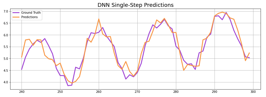
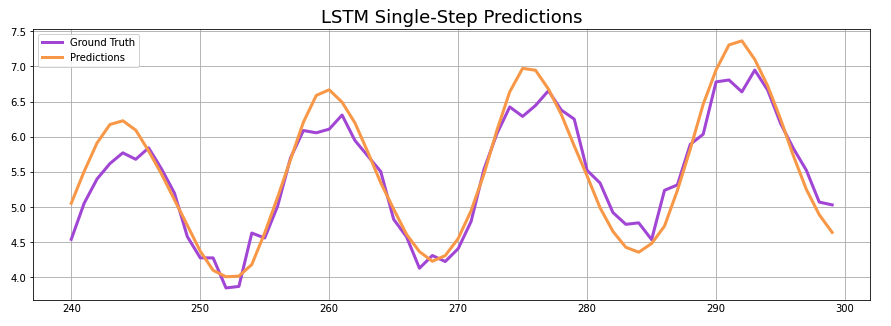
Both networks seem to have done a pretty good job matching the series, but there are some notable differences. The DNN appears to be more susceptible to the noise in the data, introducing this randomness into its forecast, while the LSTM forecasts a very smooth sine wave. While the LSTM forecast is easier on the eyes, it appears to be trending a bit below the validation set in the second half of the series.

Multi-Step Forecasting

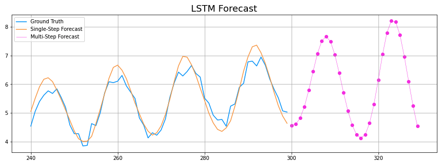
Next, let’s have both models generate forecasts using the test set to generate new time series predictions based on their existing predictions. We’ll graph these multi-step forecasts in pink, extending off of the validation forecasts we generated above.

 for time in range(0, rolling_forecast_range):
   prediction = model.predict(test_series[-window_size:][np.newaxis])
   prediction_unscaled = scaler.inverse_transform(prediction)
   test_series = np.append(test_series, prediction)
. . .
plot_forecast(dnn_multistep_forecast, df_dnn_valid_pred)
plot_forecast(lstm_multistep_forecast, df_lstm_valid_pred)

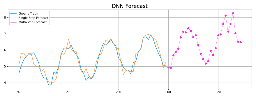
By forecasting into the unsupervised future, we can better differentiate how both networks perform. As mentioned before, the DNN predictions follow less of a consistent sine wave. However, they do appear much more accurate, as the wave amplitudes are consistent and the upward trend continues. 

Meanwhile, the LSTM forecast errors appear to amplify over time, with the wave amplitudes rapidly increasing and the upward trend being lost. While it’s less accurate overall, it does have the interesting advantage of better isolating the core sine wave from the noise. Let’s take a look at the MAE for both of these forecasts against the test data.

DNN MAE: 0.27
LSTM MAE: 0.63

As expected, the DNN’s multi-step forecast was much closer to the test set data. It’s important to note – this single comparison does very little to express the strengths and weaknesses of both types of networks. Through iteration and adjustment of parameters, both networks could yield vastly different results.

In this article, we covered how Deep Neural Networks and Long Short Term Memory Networks are constructed, and how these networks can intake and produce sequence data. We then saw that in addition to the single-step predictions we’ve made in the past, we can also generate multi-step predictions that extend into the unsupervised future.

This concludes our series on manually building networks to learn and forecast time series data. In the future, we’ll explore how AI and Machine Learning tools, such as the Microsoft Azure Anomaly Detector, can help with a variety of time series problems.

About Mission Data

We’re designers, engineers, and strategists building innovative digital products that transform the way companies do business. Learn more: https://www.missiondata.com.